Tutorial 2: Invertible Layers (Fixed Resolution)
Additive coupling layers
Additive coupling layers are simple invertible layers, which are fundamental building blocks of iUNets – although other types of layers can also easily be implemented by the user. They are conceptually similar to residual layers, and their inverse mapping can be computed just as fast as their forward mapping. In contrast to invertible learnable up- and downsampling, these preserve the resolution of their input. They are therefore used for computing features within each specific resolution of the iUNet.
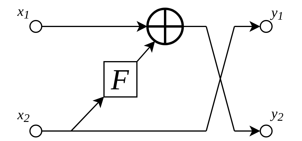
Additive coupling layers as implemented in this library. The input and output is split into two groups of channels. Here, the computational block \(F\) can be any sequence of e.g. convolutional layers with normalization. Note that the roles of \(x_1\) and \(x_2\) are reversed afterwards.
By splitting the input activation \(x\) and output activation \(y\) into two groups of channels (i.e. \((x_1, x_2) \cong x\) and \((y_1, y_2) \cong y\)), additive coupling layers define an invertible mapping \(x \mapsto y\) via
where the coupling function \(F\) is an (almost) arbitrary mapping. \(F\) just has to map from the space of \(x_2\) to the space of \(x_1\). In practice, this can for instance be a sequence of convolutional layers with batch normalization.
By default, this is one convolutional layer followed by a leaky ReLU nonlinearity and layer optimization, although the number of layers can be easily specified, as explained below.
The inverse of the above mapping is computed algebraically via
How many additive coupling layers?
Most users will first try to transfer their experience from non-invertible networks to additive coupling layers. The most comparable type of layer to additive coupling layers are probably residual layers, as they add a learnable transformation of the input to the original input. One can very roughly think of two additive coupling layers as being equivalent to one residual layer (strongly depending of course on the exact design of \(F\)).
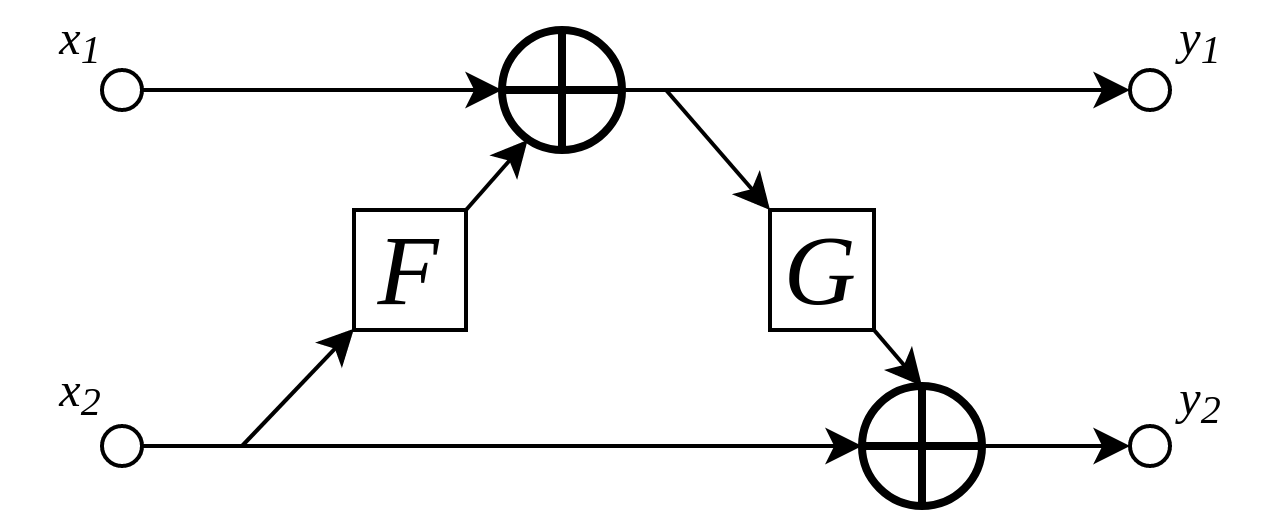
Two consecutive additive coupling layers operate on all input channels, whereas a single additive coupling layer only operates on one portion of the input channels.
Note that these ‘double’ additive coupling layers are also sometimes referred to as additive coupling layers. In this implementation, we decided to use the ‘single’ additive coupling strategy, as one essentially halves the required memory this way.
Customization options
A custom resolution-preserving invertible layer can be specified by supplying
a specific function to the iUNet via the create_module_fn keyword. This
function has to have the signature
create_module_fn(in_channels, **kwargs)
and has to return an instance of torch.nn.Module which, additionally to
its forward-method, has to implement an inverse-method. When calling the
iUNet constructor, each resolution-preserving invertible layer is then
created by a call to create_module_fn. The dafault value for
create_module_fn is iunets.layers.create_standard_module.
This can be for instance an additive coupling layer with a desired mapping
F, e.g.
import torch
from torch import nn
import iunets
from iunets.layers import AdditiveCoupling

# Define a custom additive coupling layer
def my_module_fn(in_channels, **kwargs):
    channel_split_pos = in_channels//2

    conv_layer = nn.Conv3d(in_channels = channel_split_pos,
                           out_channels = in_channels - channel_split_pos,
                           kernel_size = 3,
                           padding = 1)
    nonlinearity = nn.ReLU()
    F = nn.Sequential(conv_layer, nonlinearity)

    return AdditiveCoupling(F, channel_split_pos)

# Create a batch of random data
x = torch.randn(4, 32, 128, 128, 128).to('cuda')

# Create an instance of the above invertible layer
invertible_layer = my_module_fn(32).to('cuda')

# Compute the output of the layer and reconstruct its input
y = invertible_layer(x)
x_reconstructed = invertible_layer.inverse(y)

# Check the quality of reconstruction
print("MSE: {}".format(nn.functional.mse_loss(x, x_reconstructed).item()))
Output:
MSE: 2.5294868141494326e-16
Now we can plug the above-defined my_module_fn into an iUNet:
# Create a iUNet with create_module_fn = my_module_fn
model = iunets.iUNet(
    channels = (32,64,128),
    dim = 3,
    architecture = (2,3,4),
    create_module_fn = my_module_fn
)
model = model.to('cuda')

# Compute the output of the iUNet and reconstruct its input
y = model(x)
x_reconstructed = model.inverse(y)

# Check the quality of reconstruction
print("MSE: {}".format(nn.functional.mse_loss(x, x_reconstructed).item()))
Output:
MSE: 3.4675983872495264e-13
Additional options
By supplying a dictionary to the iUNet via module_kwargs, its values
can be consumed by create_module_fn. In the following example, the layer’s
nonlinearity can be specified via a string.
def my_customizable_module_fn(in_channels, **kwargs):
    channel_split_pos = in_channels//2
    conv_layer = nn.Conv3d(in_channels = channel_split_pos,
                           out_channels = in_channels - channel_split_pos,
                           kernel_size = 3,
                           padding = 1)
    nonlinearity_str = kwargs.get('nonlinearity', 'ReLU')
    nonlinearity = getattr(nn, nonlinearity_str)()
    F = nn.Sequential(conv_layer, nonlinearity)
    return AdditiveCoupling(F, channel_split_pos)

model = iunets.iUNet(
    channels=(32,64,128),
    dim = 3,
    architecture = (2,3,4),
    create_module_fn = my_customizable_module_fn,
    module_kwargs = {'nonlinearity': 'LeakyReLU'}
)
model = model.to('cuda')
For the default module creator iunets.layers.create_standard_module,
passable keywords are "block_depth" (which controls the number of
Conv-LReLU-Normalization-blocks, expecting an int) and zero_init
(which initializes these blocks as zeros, expecting a bool; this initializes
the whole additive coupling layer as the identity, up to the reordering of
channels).
Layerwise definition of invertible layers
When create_module_fn is called from inside the iUNet constructor, apart
from optional keywords, kwargs also automatically includes basic
information about the iUNet (dim and architecture), as well as the
coordinates of the current module. These are:
"branch", which denotes the encoder ("encoder", the downsampling branch) or the decoder ("decoder", the upsampling branch) of the iUNet
"level", which denotes the index of the resolution level inside the iUNet, where0denotes the highest resolution
"module_index", which runs from0toarchitecture[level]-1.
This allows for fine-grained control of the creation of the layers. The
following function exemplifies this. In the above examples, we had to choose
a 3D convolution operator, whereas we would have to create a completely
different function if we were to apply this to 2D data. Here, we choose the
correct convolution operator based on the value of dim. Furthermore, we add
an instance normalization layer in the very last block of the iUNet.
import numpy as np

def my_fine_grained_module_fn(in_channels, **kwargs):
    channel_split_pos = in_channels//2

    # Coordinates of the current module
    branch = kwargs.get('branch')
    level = kwargs.get('level')
    module_index = kwargs.get('module_index')

    # architecure keyword passed to the iUNet
    architecture = kwargs.get('architecture')

    # Dimensionality of the data, for choosing the right convolution
    dim = kwargs.get('dim')

    conv_op = [nn.Conv1d, nn.Conv2d, nn.Conv3d][dim-1]
    conv_layer = conv_op(in_channels = channel_split_pos,
                         out_channels = in_channels - channel_split_pos,
                         kernel_size = 3,
                         padding = 1)

    nonlinearity = nn.ReLU()
    layers = [conv_layer, nonlinearity]

    # In the very last layer, apply an instance normalization
    if (branch is 'decoder' and
        level==0 and
        module_index==architecture[0]-1):
        print(
            "Adding instance normalization in coordinate ({},{},{}).".format(
                branch, level, module_index
            )
        )

        norm_op = [nn.InstanceNorm1d, nn.InstanceNorm2d, nn.InstanceNorm3d][dim-1]
        layers.append(norm_op(channel_split_pos))

    F = nn.Sequential(*layers)
    return AdditiveCoupling(F, channel_split_pos)

model = iunets.iUNet(
    channels=(32,64,128),
    dim = 3,
    architecture = [3,4,5],
    create_module_fn = my_fine_grained_module_fn
)
model = model.to('cuda')
Output:
Adding instance normalization in coordinate (decoder,0,2).