Tutorial 3: Invertible Learnable Up- and Downsampling¶

One of the central aspects of U-Nets are up- and downsampling operations: In the encoder portion, the features are iteratively downsampled, before they are recombined with their later upsampled counterparts by channel concatenation in the decoder portion. At first, building invertible up- or downsampling layers seems nonsensical, as the resolution (and thus the dimensionality) of the input is altered.

However, if – in the case of downsampling – the number of channels is increased to make up for the loss of resolution, such that the total number of pixels/voxels remains constant after downsampling, the downsampling can be made invertible.

The following Theorem describes the concept of invertible downsampling for 2D data. The theorem is given in a more formal way (and for general \(d\)-dimensional data) in our paper.

Theorem (invertible downsampling for 2D data, informal, Pytorch nomenclature): Let \(s_1, s_2 \in \mathbb{N}\) and \(\sigma = s_1 s_2\), and let \(M\) be an orthogonal \((\sigma \times \sigma)\)-matrix. Let \(x\) be our input batch of shape \((N, 1, H, W)\), where \(H\) is divisible by \(s_1\) and \(W\) is divisible by \(s_2\) (without remainders). We now reorder the entries of \(M\) into a convolutional kernel \(K\) of shape \((\sigma, 1, s_1, s_2)\) in a specific way. Then the convolution of \(x\) with the kernel \(K\) using a stride of \((s_1,s_2)\) produces an output \(y\) of shape \((N, \sigma, H/s_1, W/s_2)\). This operation can be inverted by applying the associated transpose convolution with kernel \(K\) to \(y\).

This concept can be easily extended to general input batches with \(C\) channels by applying this to each input channel independently. The inverse operation to invertible downsampling (via a transposed strided convolution) realizes invertible upsampling.

An introductory example¶

The following example requires the package skimage to load the example image.

import numpy as np
from skimage import data
from matplotlib import pyplot as plt

import torch
from iunets.layers import InvertibleDownsampling2D

# Load example image
img = np.array(data.camera(), dtype=np.float32) / 255.

# Display input image
plt.figure(figsize=(7,7),constrained_layout=True)
plt.imshow(img, cmap='Greys_r')

# Helper functions to transfer between Numpy and Pytorch
to_torch = lambda img: torch.Tensor(np.expand_dims(img, (0,1)))
to_numpy = lambda img: img.detach().numpy()

# Transfer to Torch, reshape to batch of shape (1, 1, 512, 512)
torch_img = to_torch(img)

# Create learnable invertible downsampling layer
downsampling = InvertibleDownsampling2D(
    in_channels=1,
    stride=(2,2)
)

# Compute downsampled images
output = downsampling(torch_img)
output = to_numpy(output)

# Display output images
fig = plt.figure(figsize=(7,7),constrained_layout=True)
ax_array = fig.subplots(2, 2, squeeze=False)
ax_array[0, 0].imshow(output[0,0], cmap='Greys_r')
ax_array[0, 1].imshow(output[0,1], cmap='Greys_r')
ax_array[1, 0].imshow(output[0,2], cmap='Greys_r')
ax_array[1, 1].imshow(output[0,3], cmap='Greys_r')

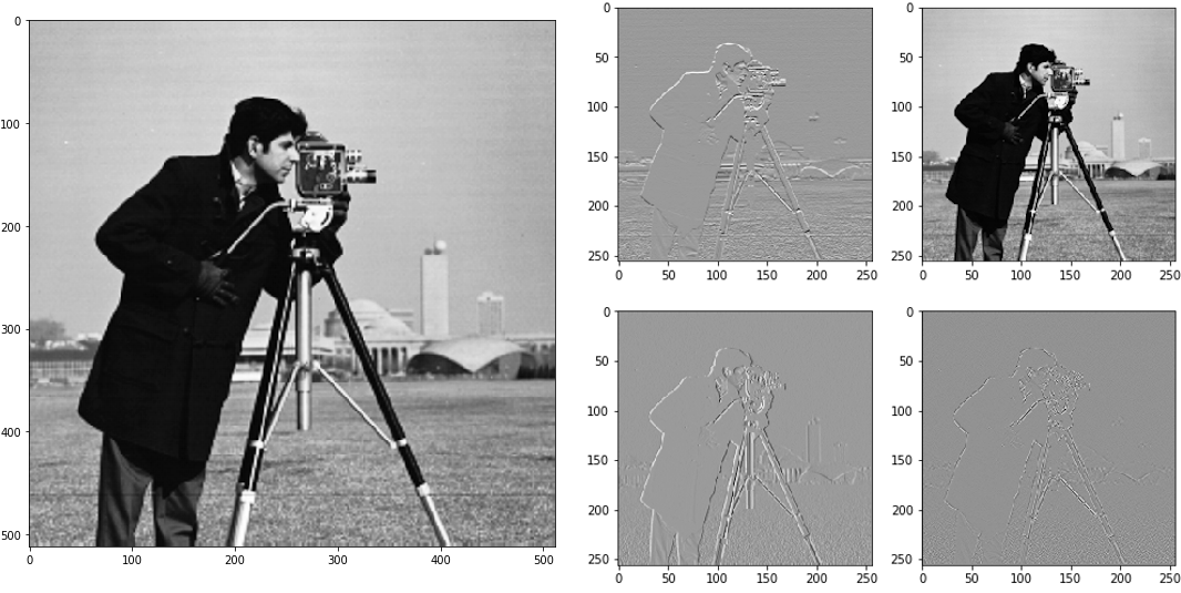
The example image after invertibly downsampling with a stride of (2,2). By default, this is initialized as the Haar transform.¶

We now check how well the inversion works:

img_reconstruction = downsampling.inverse(downsampled)
print("MSE: {}".format(torch.nn.functional.mse_loss(torch_img, img_reconstruction).item()))

Output:

MSE: 1.0410113272302972e-15

Invertible up- and downsampling in iUNets¶

The behavior of the invertible up- and downsampling operations can be controlled in the iUNet constructor.

from iunets import iUNet
model = iUNet(
    channels=(32,64,128,256),
    dim=3,
    architecture=(2,2,2,2),
    resampling_stride=2,
    resampling_method='exp',
    resampling_init='haar',
    resampling_kwargs={}
)
model.print_layout()

Output:

32-32-(24/8)----------------------------------------------------(24/8)-32-32
---------64-64-(48/16)--------------------------------(48/16)-64-64---------
------------------128-128-(96/32)---------(96/32)-128-128-------------------
------------------------------256-256--256-256------------------------------

The relevant keywords are:

resampling_stride, which controls the amount of spatial down-/upsampling and hence the channel multiplier. In the following section, further details are given.

resampling_method, which controls the parametrization method for (special) orthogonal matrices. Current options are "exp", "cayley" and "householder".

"cayley": Cayley transform of a skew-symmetric matrix

"exp": matrix exponential of a skew-symmetric matrix

"householder": a product of Householder matrices

resampling_init, which controls the initialization. Current options are "haar", "squeeze", "random" or a user-specified torch.Tensor or numpy.ndarray.

resampling_kwargs, which can be used to provide additional keywords. Currently only used if Householder transforms are used for parametrization, in which case "n_reflections" controls the number of Householder reflections (defaults to using all possible reflections).

Currently only used if Householder transforms are used for parametrization, in which case "n_reflections" controls the number of Householder reflections (defaults to using all possible reflections).

Anisotropic up- and downsampling¶

Very often, medical imaging data is not exactly cube-shaped. This can for example be the case when only a few consecutive slices in z-direction of a CT image are considered. In these cases, it makes sense to apply fewer (or less extreme) downsampling operators to these smaller axes. With the keyword resampling_stride, the (up- and) downsampling strides can be controlled exactly, in order to achieve the desired anisotropic downsampling. The format can be either a single integer, a single tuple (where the length corresponds to the spatial dimensions of the data), or a list containing either of the last two options (where the length of the list has to be equal to the number of downsampling operations), e.g.

resampling_stride=2 will result in a downsampling factor of 2 in each coordinate, for each up- and downsampling operation.
resampling_stride=(2,1,3) will result in downsampling factors (2,1,3) along Pytorch’s (z,y,x)-coordinate system for each up- and downsampling operation.
resampling_stride=[(2,1,3), 2, (4,3,1)] will use
- factors (2,1,3) in the first downsampling operation
- factor 2 along each coordinate in the second downsampling operation
- factors (4,3,1) in the third downsampling operation
- This also applies to the respective upsampling operations in the decoding portion of the iUNet.
- Note that this (resolution-specific) setting requires len(architecture)==4.

Channel multipliers and slicing behavior¶

The change in the number of channels when performing invertible up- or downsampling is inherently tied to the up-/downsampling factors, i.e. the resampling_stride. The factor by which the number of channels is multiplied respectively divided is called the channel multiplier (\(\sigma\) in the above introduction).

For example in 3D, a downsampling stride of 2 in all directions (i.e. resampling_stride=2) results in a channel multiplier of 8. However, the number of channels does not increase by this factor of 8 with each decreasing resolution level: This is because invertibly downsampling a pre-specified number of channels gets sliced off (for later re-concatenation in the decoding portion of the iUNet). The number of sliced-off channels thus determines the factor by which the number of channels changes in each resolution level.

This means that not any specific setting for channels can be enforced. Instead, here we automatically choose the best possible approximation to the intended choice of channels.

Example:

model = iUNet(
    channels=(3,25,32,55,128),
    dim=3,
    architecture=(2,2,2,2,2),
    resampling_stride=[(1,2,3),(2,2,2),(5,1,2),2]
)
model.print_layout()

print("Channel multipliers: {}".format(model.channel_multipliers))
print("Downsampling factors: {}".format(model.downsampling_factors))

Output:

Could not exactly create an iUNet with channels=(3, 25, 32, 55, 128)
and resampling_stride=[(1, 2, 3), (2, 2, 2), (5, 1, 2), (2, 2, 2)].
Instead using closest achievable configuration: channels=(3, 12, 32, 60, 128).
Average relative error: 0.1527

3-3-(1/2)-----------------------------------------------------------------(1/2)-3-3
------12-12-(8/4)------------------------------------------------(8/4)-12-12-------
---------------32-32-(26/6)-----------------------------(26/6)-32-32---------------
------------------------60-60-(44/16)---------(44/16)-60-60------------------------
---------------------------------128-128--128-128----------------------------------

Channel multipliers: [6, 8, 10, 8]
Downsampling factors: (20, 8, 24)

Here, the channel multipliers are the products of the resampling factors over all spatial dimensions (e.g. 1*2*3=6 for the first downsampling operation), whereas the downsampling factors denote, by how much the input data is downsampled in total (e.g. 1*2*5*2=20 for the first coordinate).